Effective Handling of Geospatial Data in DynamoDB
Handling Geospatial data in DynamoDB doesn’t feel like a natural fit, and can appear complex. With the right approach and some upfront work, you can leverage the unique powers of DynamoDB for your geospatial application.
There are some really good existing patterns for handling geospatial data, in particular the DynamoDB Geo Package. However, there are some limitations I wanted to avoid for my application. In particular, I wanted more control over the structure of my data, and I wanted to be able to return a geographically distributed set of results within a large result set without paginating.
This article walks through how I achieved this using DynamoDB, with an example dataset of weather data from ~5,000 global airports. The approach for structuring and querying the geospatial data includes making use of multiple geohash indexes and some de-clustering.
The end goal:
- Real-time queries working at lightning speed at any precision level
- Uniform response time, regardless of the bounding box size
- Queries not impacted by the total dataset size: No scan operations, only optimised queries.
- A random, well-distributed set of results, rather than clustered data from a single corner of the bounding box
Introduction
The code for this article can be found here:
👉 GitHub Repository – DynamoDB Geospatial Example
The project demonstrates how to:
- Load real-world weather data into DynamoDB
- Structure indexes for multi-level geohash precision
- Support both large (worldwide) and small (town-level) bounding box queries
- Perform “points of interest along a route” type queries
- Return randomised results evenly distributed across space
The Challenge with Geospatial in DynamoDB
At its core, DynamoDB does not provide geospatial queries natively. You cannot simply say: “Give me all points within this bounding box.”
We need to break the problem down:
- Geohashing: Encode latitude and longitude into a compact, ordered string.
- Precision levels: Wider bounding boxes use low-precision geohashes, smaller bounding boxes use higher precision.
- Indexes: Leverage DynamoDB Primary Partition and GSIs to query data at the right level of precision.
- Partition prefixes: Avoid hot partitions and enable randomised selection.
Table Design
Here’s the design I used that allows for multi-precision level queries:
| Partition Key | Sort Key | GSI1 Partition Key | GSI1 Sort Key |
|---|---|---|---|
| PK | SK | GSI1PK | GSI1SK |
<ShardID>#<GeoHash Precision 1> |
<GeoHash Precision 8> |
<GeoHash Precision 4> |
<GeoHash Precision 8> |
And importantly:
- The
ShardIDis a random number (1–10 in the default case) that distributes data across partitions. - We fan out to parallel queries, returning a random spread of results.
The precision levels configurable based on your use case, but under test, I found this structure to work well from very low to very high precision queries.
The ShardID is used on the main partition key, while the GSI1 allows for mid-level precision queries without the shard. This provides two benefits:
- We don’t create a hot partition when using a very low precision geohash (e.g. world-level queries) on the main partition key.
- We are able to make higher precision queries (e.g. city-level) without needing to include the shard, which would require multiple queries to cover all shard values.
Query Types
Depending on the zoom level of the bounding box, we dynamically adjust which keys/indexes are used:
- PK only → World-scale queries
- PK + SK → Country or region queries
- GSI1PK only → City-level queries
- GSI1PK + GSI1SK → Town-level queries
This tiered approach ensures we always query at the right precision without over-fetching.
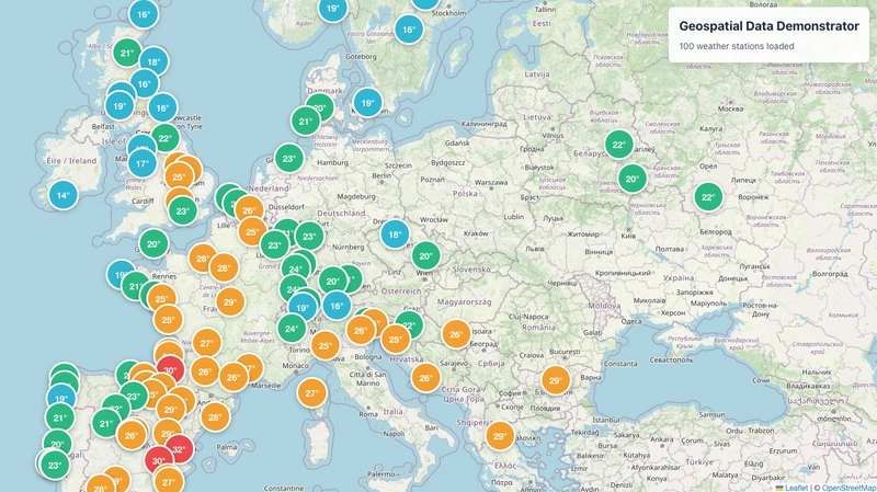
Randomised Result Distribution
Without a partition prefix, DynamoDB queries naturally return clustered results (e.g. all from the “top-left” corner). By introducing a random ShardID prefix, we ensure queries fan out across partitions and return a spread of points across the bounding box.
Sharding alone doesn’t completely solve the clustering issue, especially for large bounding boxes with low precision geohashes. Therefore we further randomise results by gridding the bounding box into smaller sections and selecting results evenly from these grids.
⚠️ Before Querying world-scale without gridding → clustered data:
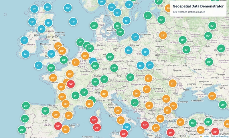
✅ After Querying world-scale with partition prefixes and gridding → evenly spread data:
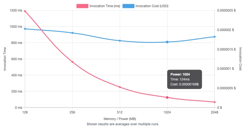
Performance Tuning with Lambda
Response times were tested response times using the truly execelent Lambda Power Tuning.
At 1024MB, with large (county level) bounding box queries averaged ~124ms. Scaling memory up or down adjusted response time linearly without any unpredictable spikes.
Example: Bounding Box Queries
Here’s a comparison of bounding box sizes, the index used, and the performance on my ~5,000 record dataset:
| Level | Bounding Box | Diagonal Distance (Km) | Geohash Precision | Index Used | DDB Queries Made | Avg Response Time (1024MB) |
|---|---|---|---|---|---|---|
| World | (80, -170), (-80, 170) | 17,845 km | 1 | PK | 320 | 880 ms |
| Continent | (70, -25), (40, 30) | 4,568 km | 1 | PK | 40 | 150 ms |
| Country | (43, -10), (37, 2) | 1,220 km | 2 | PK + SK | 40 | 124 ms |
| Region | (50, 8), (47, 13) | 497 km | 3 | PK + SK | 150 | 324 ms |
| City | (51.6, -0.45), (51.3, 0.2) | 56 km | 4 | GSI1 | 9 | 23 ms |
| Town | (37.041, -7.995), (37.006, -7.901) | 9 km | 4 | GSI1PK + GSI1SK | 3 | 11 ms |
Even world-scale queries return results in under a second, with evenly distributed points. There is also much more we could do here to optimise the Lambda function performance.
This shows the approach delivers uniform response times regardless of bounding box size.
Getting Started
To get started with the example project:
- Clone the repo
- Deploy the CDK stack (see README)
- Load the sample dataset (5,000 airports with METAR weather data)
- Load up the frontend and try different bounding box queries
You’ll see that whether querying the whole world or a small town, response times remain fast and results are evenly distributed.
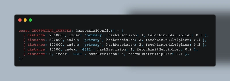
Configuration
The hashes and indexes used as configured within the environment configuration: config/environment-config.ts and queries configuration are configured within the config/geospatial-config.ts which includes the indexes and precision that should be used based on the size of the bounding box.
Architecture
The demo project consists of two main components:
- Frontend: React-based web application served via CloudFront. Deployed with AWS CDK.
- Backend: Serverless API built with AWS Lambda and API Gateway, using DynamoDB for data storage and event driven architecture for real-time updates. Deployed with AWS CDK.
AWS services consist of:
- Amazon DynamoDB for geospatial data store
- AWS Lambda for serverless compute
- AWS API Gateway for REST API management
- Amazon S3 for static hosting of the frontend
- Amazon CloudFront for content delivery
API
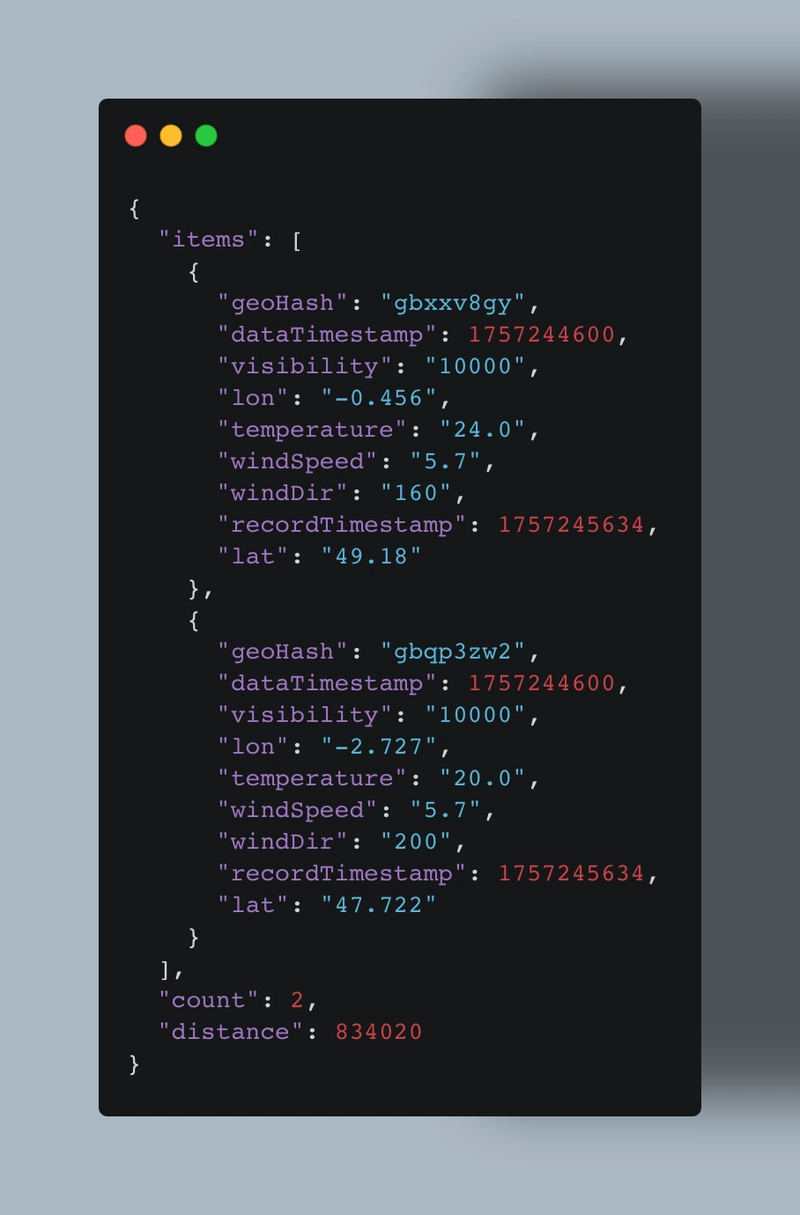
The API also includes a route endpoint that uses similar logic to the bounding box query and will return points of interest along a route. The payload response will including the total distance of the route:
Next Steps
This approach provides a solid foundation for handling geospatial data in DynamoDB:
- Scalable to millions of records
- Uniform response times
- Randomised and well-distributed query results
Future work could include:
- Additional GSIs for intermediate precision levels
- Support for more complex geospatial queries (e.g. radius, nearest neighbor)
- Improved efficiency of the de-clustering. This is currently a very basic approach, and could be improved with more advanced algorithms.
About Me
I’m Ian, an AWS Serverless Specialist, AWS Community Builder and AWS Certified Cloud Architect based in the UK. I work as an independent consultant, having worked across multiple sectors, with a passion for Aviation.
Let’s connect on LinkedIn, or find out more about my work at Crockwell Solutions.